Unification

Operationally the query age P 23 is unified with each and every rule present in the program starting from the first one.

Unification compares two terms structurally and eventually assigns variables. For example for the first rule of the program we obtain the following unification problem:

age P 23 = age mallory 23

This problem can be simplified into smaller unification problems following the structure of the terms:

age = age
P = mallory
23 = 23

The first and last are trivial, while the second one can be satisfied by assigning mallory to P. All equations are solved, hence unification succeeds.

See also the Wikipedia page on Unification.

Since the first part of the query is succesful the rest of the query is run: the value of P is printed as well as the "is 23 years old" string.

A = 23, age P A, Msg = "is 23 years old", coq.say P Msg

Let's try a query harder to solve!

Elpi Query lp:{{

  age P 20, coq.say P "is 20 years old"

}}.
alice is 20 years old
Query assignments:
P = alice

This time the unification problem for the first rule in the program is:

age P 20 = age mallory 23

that is simplified to:

age = age
P = mallory
20 = 23

The second equation can be solved by assigning mallory to P, but the third one has no solution, so unification fails.

Backtracking

When failure occurs all assignements are undone (i.e. P is unset again) and the next rule in the program is tried. This operation is called backtracking.

The unification problem for the next rule is:

age P 20 = age bob 23

This one also fails. The unification problem for the last rule is:

age P 20 = age alice 20

This one works, and the assigment P = alice is kept as the result of the first part of the query. Then P is printed and the program ends.

An even harder query is the following one where we ask for two distinct individuals to have the same age.

Elpi Query lp:{{

  age P A, age Q A, not(P = Q),
  coq.say P "and" Q "are" A "years old"

}}.
mallory and bob are 23 years old
Query assignments:
A = 23
P = mallory
Q = bob

This example shows that backtracking is global. The first solution for age P A and age Q A picks P and Q to be the same individual mallory, but then not(P = Q) fails and forces the last choice that was made to be reconsidered, so Q becomes bob.

Look at the output of the following code to better understand how backtracking works.

Elpi Query lp:{{

   age P A, coq.say "I picked P =" P,
   age Q A, coq.say "I picked Q =" Q,
   not(P = Q),
   coq.say "the last choice worked!",
   coq.say P "and" Q "are" A "years old"

}}.
I picked P = mallory
I picked Q = mallory
I picked Q = bob
the last choice worked!
mallory and bob are 23 years old
Query assignments:
A = 23
P = mallory
Q = bob

Facts and conditional rules

The rules we have seen so far are facts: they always hold. In general rules can only be applied if some condition holds. Conditions are also called premises, we may use the two terms interchangeably.

Here we add to our program a rule that defines what older P Q means in terms of the age of P and Q.

Elpi Accumulate lp:{{

  pred older o:person, o:person.
  older P Q :- age P N, age Q M, N > M.

}}.

The rule reads: P is older than Q if N is the age of P and M is the age of Q and N is greater than M.

Let's run a query using older:

Elpi Query lp:{{

  older bob X,
  coq.say "bob is older than" X

}}.
bob is older than alice
Query assignments:
X = alice

The query older bob X is unified with the head of the program rule older P Q assigning P = bob and X = Q. Then three new queries are run:

age bob N
age Q M
N > M

The former assigns N = 23, the second one first sets Q = mallory and M = 23. This makes the last query to fail, since 23 > 23 is false. Hence the second query is run again and again until Q is set to alice and M to 20.

Variables in the query are said to be existentially quantified because Elpi will try to find one possible value for them.

Conversely, the variables used in rules are universally quantified in the front of the rule. This means that the same program rule can be used multiple times, and each time the variables are fresh.

In the following example the variable P in older P Q :- ... once takes bob and another time takes mallory.

Elpi Query lp:{{

  older bob X, older mallory X,
  coq.say "both bob and mallory are older than" X

}}.
both bob and mallory are older than alice
Query assignments:
X = alice

λ-abstraction

Functions built using λ-abstraction can be applied to arguments and honor the usual β-reduction rule (the argument is substituted for the bound variable).

In the following example F 23 reads, once the β-reduction is performed, age alice 23.

Elpi Query lp:{{

  F = (x\ age alice x),
  coq.say "F =" F,
  coq.say "F 20 =" (F 20),
  coq.say "F 23 =" (F 23)

}}.
F = c0 \ age alice c0
F 20 = age alice 20
F 23 = age alice 23
Query assignments:
  F = c0 \
age alice c0

Let's now write the "hello world" of λProlog: an interpreter and type checker for the simply typed λ-calculus. We call this program stlc.

We start by declaring that term is a type and that app and fun are constructors of that type.

Elpi Program stlc lp:{{

  kind  term  type.

  type  app   term -> term -> term.
  type  fun   (term -> term) -> term.

}}.

The constructor app takes two terms while fun only one (of functional type).

Note that

• there is no constructor for variables, we will use the notion of bound variable of λProlog in order to represent variables
• fun takes a function as subterm, i.e. something we can build using the λ-abstraction x\ ...

As a consequence, the identity function λx.x is written like this:

fun (x\ x)

while the first projection λx.λy.x is written:

fun (x\ fun (y\ x))

Another consequence of this approach is that there is no such thing as a free variable in our representation of the λ-calculus. Variables are only available under the λ-abstraction of the programming language, that gives them a well defined scope and substitution operation (β-reduction).

This approach is called HOAS.

We can now implement weak head reduction, that is we stop reducing when the term is a fun or a global constant (potentially applied). If the term is app (fun F) A then we compute the reduct F A. Note that F is a λProlog function, so passing an argument to it implements the substitution of the actual argument for the bound variable.

We first give a type and a mode for our predicate whd. It reads "whd takes a term in input and gives a term in output". We will explain what input means precisely later, for now just think about it as a comment.

Elpi Accumulate lp:{{

  pred whd i:term, o:term.

  % when the head "Hd" of an "app" (lication) is a
  % "fun" we substitute and continue
  whd (app Hd Arg) Reduct :- whd Hd (fun F), !,
    whd (F Arg) Reduct.

  % otherwise a term X is already in normal form.
  whd X Reduct :- Reduct = X.

}}.

Recall that, due to backtracking, all rules are potentially used. Here whenever the first premise of the first rule succeeds we want the second rule to be skipped, since we found a redex.

The premises of a rule are run in order and the ! operator discards all other rules following the current one. Said otherwise it commits to the currently chosen rule for the current query (but leaves all rules available for subsequent queries, they are not erased from the program). So, as soon as whd Hd (fun F) succeeds we discard the second rule.

Elpi Query lp:{{

  I = (fun x\x),
  whd I T, coq.say "λx.x ~>" T,
  whd (app I I) T1, coq.say "(λx.x) (λx.x) ~>" T1

}}.
λx.x ~> fun c0 \ c0
(λx.x) (λx.x) ~> fun c0 \ c0
Query assignments:
I = fun c0 \ c0
T = fun c0 \ c0
T1 = fun c0 \ c0

Another little test using global constants:

Elpi Accumulate lp:{{

  type foo, bar term.

}}.

Elpi Query lp:{{

  Fst = fun (x\ fun y\ x),
  T = app (app Fst foo) bar,
  whd T T1, coq.say "(Fst foo bar) ~>" T1,
  S = app foo bar,
  whd S S1, coq.say "(foo bar) ~>" S1

}}.
(Fst foo bar) ~> foo
(foo bar) ~> app foo bar
Query assignments:
Fst = fun c0 \ fun c1 \ c0
S = app foo bar
S1 = app foo bar
T = app (app (fun c0 \ fun c1 \ c0) foo) bar
T1 = foo

A last test with a lambda term that has no weak head normal form:

Elpi Bound Steps 1000. (* Let's be cautious *)
Elpi Query lp:{{

  Delta = fun (x\ app x x),
  Omega = app Delta Delta,
  whd Omega Hummm, coq.say "not going to happen"

}}.
elpi run out of steps (1000)
Elpi Bound Steps 0.

pi x\ and =>

We have seen how to implement subtitution using the binders of λProlog. More often than not we need to move under binders rather than remove them by substituting some term in place of the bound variable.

In order to move under a binder and inspect the body of a function λProlog provides the pi quantifier and the => connective.

A good showcase for these features is to implement a type checker for the simply typed lambda calculus. See also the Wikipedia page on the simply typed lambda calculus.

We start by defining the data type of simple types. We then declare a new predicate of (for "type of") and finally we provide two rules, one for each term constructor.

Elpi Accumulate lp:{{

  kind  ty   type.           % the data type of types
  type  arr  ty -> ty -> ty. % our type constructor

  pred of i:term, o:ty. % the type checking algorithm

  % for the app node we ensure the head is a function from
  % A to B, and that the argument is of type A
  of (app Hd Arg) B :-
    of Hd (arr A B), of Arg A.

  % for lambda, instead of using a context (a list) of bound
  % variables we use pi and => , explained below
  of (fun F) (arr A B) :-
    pi x\ of x A => of (F x) B.

}}.

The pi name\ code syntax is reserved, as well as rule => code.

Operationally pi x\ code introduces a fresh constant c for x and then runs code. Operationally rule => code adds rule to the program and runs code. Such extra rule is said to be hypothetical. Both the constant for x and rule are removed once code terminates.

Note that in this last example the hypothetical rule is going to be of c A for a fixed A and a fresh constant c. The variable A is fixed but not assigned yet, meaning that c has a type, and only one, but we may not know it yet.

Now let's assign a type to λx.λy.x:

Elpi Query lp:{{

of (fun (x\ fun y\ x)) Ty, coq.say "The type of λx.λy.x is:" Ty

}}.
The type of λx.λy.x is: arr X0 (arr X1 X0)
Query assignments:
Ty = arr X0 (arr X1 X0)

Let's run this example step by step:

The rule for fun is used:

• arrow A1 B1 is assigned to Ty by unification
• the pi x\ quantifier creates a fresh constant c1 to play the role of x
• the => connective adds the rule of c1 A1 the program
• the new query of (fun y\ c1) B1 is run.

Again, the rule for fun is used (since its variables are universally quantified, we use A2, B2... this time):

• arrow A2 B2 is assigned to B1 by unification
• the pi x\ quantifier creates a fresh constant c2 to play the role of x
• the => connective adds the rule of c2 A2 the program
• the new query of c1 B2 is run.

The (hypotetical) rule of c1 A1 is used:

• unification assigns A1 to B2

The value of Ty is hence arr A1 (arr A2 A1), a good type for λx.λy.x (the first argument and the output have the same type A1).

What about the term λx.(x x) ?

Elpi Query lp:{{

  Delta = fun (x\ app x x),
  (of Delta Ty ; coq.say "Error:" Delta "has no type")

}}.
Error: fun c0 \ app c0 c0 has no type
Query assignments:
Delta = fun c0 \ app c0 c0
Ty = X0

The ; infix operator stands for disjunction. Since we see the message of failed: the term fun (x\ app x x) is not well typed.

First, the rule for elpi:fun is selected:

• arrow A1 B1 is assigned to Ty by unification
• the pi x\ quantifier creates a fresh constant c1 to play the role of x
• the => connective adds the rule of c1 A1 the program
• the new query of (app c1 c1) B1 is run.

Then it's the turn of typing the application:

• the query of c1 (arr A2 B2) assignes to A1 the value arr A2 B2. This means that the hypothetical rule is now of c1 (arr A2 B2).

• the query of c1 A2 fails because the unification

  of c1 A2 = of c1 (arr A2 B2)
  

  has no solution, in particular the sub problem A2 = (arr A2 B2) fails the so called occur check.

Constraint Handling Rules

A constraint (handling) rule can see the store of syntactic constraints as a whole, remove constraints and/or create new goals:

Elpi Accumulate lp:{{

constraint even odd {
  % if two distinct, conflicting, constraints about the same X
  % are part of the constraint store
  rule (even X) (odd X) <=>
   % generate the following goal
   (coq.say X "can't be even and odd at the same time", fail).
}

}}.

Elpi Query lp:{{ even (s X), odd (s X) }}.
X0 can't be even and odd at the same time
The elpi tactic/command peano3 failed without giving a
specific error message. Please report this
inconvenience to the authors of the program.

See also the Wikipedia page on Constraint Handling Rules for an introduction to the sub language to manipulate constraints.

Spilling (relation composition)

Chaining "relations" can be painful, especially when they look like functions. Here we use std.append and std.rev to build a palindrome:

Elpi Program function lp:{{

pred make-palindrome i:list A, o:list A.

make-palindrome L Result :-
  std.rev L TMP,
  std.append L TMP Result.

}}.

Elpi Query lp:{{

  make-palindrome [1,2,3] A

}}.
Query assignments:
A = [1, 2, 3, 3, 2, 1]

The make-palindrome predicate has to use a temporary variable just to pass the output of a function as the input to another function.

Spilling is a syntactic elaboration which does that for you. Expressions between { and } are said to be spilled out and placed just before the predicate that contains them.

Elpi Accumulate lp:{{

pred make-palindrome2 i:list A, o:list A.

make-palindrome2 L Result :-
  std.append L {std.rev L} Result.

}}.

Elpi Query lp:{{

  make-palindrome2 [1,2,3] A

}}.
Query assignments:
A = [1, 2, 3, 3, 2, 1]

The two versions of make-palindrome are equivalent. Actually the latter is elaborated into the former.

APIs for built-in data

Functions about built-in data types are available via the calc predicate or its infix version is. Example:

Elpi Query lp:{{

   calc ( "result " ^ "=" ) X,
   Y is 3 + 2,
   coq.say X Y 

}}.
result = 5
Query assignments:
X = result =
Y = 5

The calc predicate works nicely with spilling:

Elpi Query lp:{{ coq.say "result =" {calc (2 + 3)} }}.
result = 5
Query assignments:
Spilled_1 = 5

Allocation of variables

The language let's one use λ-abstraction also to write anonymous rules but one has to be wary of where variables are bound (allocated really).

In our example we use the higher order predicate std.map:

pred std.map i:list A, i:(A -> B -> prop), o:list B.

type std.map list A -> (A -> B -> prop) -> list B -> prop.

The type of the second argument of std.map is the one of a predicate relating A with B.

Let's try to call std.map passing an anonymous rule (as we would do in a functional language by passing an anonymous function):

Elpi Accumulate lp:{{

pred bad i:list int, o:list int.

bad L Result :-
  std.map L (x\ r\ TMP is x + 1, r = TMP) Result.

pred good i:list int, o:list int.
good L Result :-
  std.map L good.aux Result.
good.aux X R :- TMP is X + 1, R = TMP.

pred good2 i:list int, o:list int.
good2 L Result :-
  std.map L (x\ r\ sigma TMP\ TMP is x + 1, r = TMP) Result.

}}.

Elpi Query lp:{{

  not(bad [1,2,3] R1),
  good [1,2,3] R2,
  good2 [1,2,3] R3

}}.
Query assignments:
R1 = X0
R2 = [2, 3, 4]
R3 = [2, 3, 4]

The problem with bad is that TMP is fresh each time the rule is used, but not every time the anonymous rule passed to map is used. Technically TMP is quantified (allocated) where L and Result are.

There are two ways to quantify TMP correctly, that is inside the anonymous predicate. One is to actually name the predicate. Another one is to use the sigma x\ quantifier to allocate TMP at every call. We recommend to name the auxiliary predicate.

One last way to skin the cat is to use => as follows. It gives us the occasion to clarify further the scope of variables.

Elpi Accumulate lp:{{

pred good3 i:list int, o:list int.
good3 L Result :-
  pi aux\
    (pi TMP X R\ aux X R :- TMP is X + 1, R = TMP) =>
    std.map L aux Result.

}}.

Elpi Query lp:{{

  good3 [1,2,3] R

}}.
Query assignments:
R = [2, 3, 4]

In this case the auxiliary predicate aux is only visible inside good3. What is interesting to remark is that the quantifications are explicit in the hypothetical rule, and they indicate clearly that each and every time aux is used TMP, X and R are fresh.

The pi x\ quantifier is dual to sigma x\ : since here it occurs negatively it has the same meaning. That is, the hypothetical rule could be written pi X R\ aux X R :- sigma TMP\ TMP is X + 1, R = TMP.

Rules = [ one-more-rule | ExtraRules ], Rules => code

The last remark worth making is that bound variables are intimately related to universal quantification, while unification variables are related to existential quantification. It goes without saying that the following two formulas are not equivalent and while the former is trivial the latter is in general false:

Let's run these two corresponding queries:

Elpi Query lp:{{ pi x\ sigma Y\ Y = x, coq.say "Y =" Y }}.
Y = c0
Elpi Query lp:{{ sigma Y\ pi x\ Y = x, coq.say "Y =" Y }}.
The elpi tactic/command function failed without giving
a specific error message. Please report this
inconvenience to the authors of the program.

Another way to put it: x is in the scope of Y only in the first formula since it is quantified before it. Hence x can be assigned to Y in that case, but not in the second query, where it is quantified after.

More in general, λProlog tracks the bound variables that are in scope of each unification variable. There are only two ways to put a bound variable in the scope:

• quantify the unification variable under the bound one (first formula)

• pass the bound variable to the unification variable explicitly: in this case the unification variable needs to have a functional type. Indeed \(\exists Y, \forall x, (Y x) = x\) has a solution: Y can be the identity function.

  Elpi Query lp:{{ sigma Y\ pi x\ Y x = x, coq.say "Y =" Y }}.
  Y = c1 \ c1

If we look again at the rule for type checking λ-abstraction:

of (fun F) (arr A B) :-
  pi x\ of x A => of (F x) B.

we can see that the only unification variable that sees the fresh x is F, because we pass x to F explicitly (recall all unification variables such as F, A, B are quantified upfront, before the pi x\ ). Indeed when we write:

on paper, the variable denoted by x being bound there can only occur in \(f\), not in \(\Gamma\) or \(B\) for example (although a different variable could be named the same, hence the usual freshness side conditions which are not really necessary using HOAS).

Remark that in the premise the variable \(x\) is still bound, this time not by a λ-abstraction but by the context \(\Gamma, x : A\). In λProlog the context is the set of hypothetical rules and pi\ -quantified variables and is implicitly handled by the runtime of the programming language.

A slogan to keep in mind is that:

Indeed the variable bound by the λ-abstraction (of our data) is replaced by a fresh variable bound by the context (of our program). This is called binder mobility. See also the paper Mechanized metatheory revisited by Dale Miller which is an excellent introduction to these concepts.

Trace browser

In order to generate a trace one needs to execute the Elpi Trace Browser. command and then run any Elpi code.

(* Elpi Trace Browser. *)

Elpi Query stlc lp:{{ % We run the query in the stlc program

  of (fun (x\ fun y\ x)) Ty, coq.say Ty

}}.
arr X0 (arr X1 X0)
Query assignments:
Ty = arr X0 (arr X1 X0)

The trace file is generated in /tmp/traced.tmp.json. If it does not load automatically one can do it manually by clicking on the load icon, in the upper right corner of the Elpi Tracer panel.

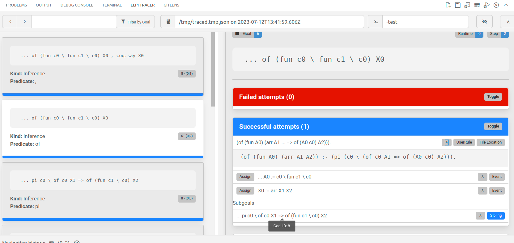
The trace browser displays, on the left column, a list of cards corresponding to a step perfoemd by the interpreter. The right side of the panel gives more details about the selected step. In the image below one can see the goal, the rule being applied, the assignments performed by the unification of the rule's head with the goal, the subgoals generated.

One can also look at the trace in text format (if VSCode is not an option, for example).

Elpi Trace.

Elpi Query stlc lp:{{ % We run the query in the stlc program

  of (fun (x\ fun y\ x)) Ty, coq.say Ty

}}.
run 1 {{{  
rid:0 step:1 gid:6 user:curgoal = , 
                                  of (fun c0 \ fun c1 \ c0) X0 , coq.say X0 
rid:0 step:1 gid:6 user:rule = and 
rid:0 step:1 gid:6 user:subgoal = 7 
rid:0 step:1 gid:7 user:newgoal = of (fun c0 \ fun c1 \ c0) X0 
rid:0 step:1 gid:6 user:subgoal = 8 
rid:0 step:1 gid:8 user:newgoal = coq.say X0 
rid:0 step:1 gid:6 user:rule:and = success 
}}} ->  (0.000s)
run 2 {{{  
rid:0 step:2 gid:7 user:curgoal = of 
                                  of (fun c0 \ fun c1 \ c0) X0 
rid:0 step:2 gid:7 user:rule = backchain 
rid:0 step:2 gid:7 user:rule:backchain:candidates = File "(stdin)", line 15, column 3, character 459: 
}}} ->  (0.000s)
select 3 {{{  
rid:0 step:2 gid:7 user:rule:backchain:try = File "(stdin)", line 15, column 3, character 459: 
                                             (of (fun A0) (arr A1 A2)) :- (
                                              pi (c0 \
                                               (of c0 A1 => of (A0 c0) A2))). 
rid:0 step:2 gid:0 user:assign = A0 := c0 \
                                 fun c1 \ c0 
rid:0 step:2 gid:0 user:assign = X0 := arr X1 X2 
rid:0 step:2 gid:7 user:subgoal = 9 
rid:0 step:2 gid:9 user:newgoal = pi c0 \ of c0 X1 => of (fun c1 \ c0) X2 
rid:0 step:2 gid:9 user:rule:backchain = success 
}}} ->  (0.000s)
run 3 {{{  
rid:0 step:3 gid:9 user:curgoal = pi 
                                  pi c0 \ of c0 X1 => of (fun c1 \ c0) X2 
rid:0 step:3 gid:9 user:rule = pi 
rid:0 step:3 gid:9 user:subgoal = 10 
rid:0 step:3 gid:10 user:newgoal = of c0 X1 => of (fun c1 \ c0) X2 
rid:0 step:3 gid:10 user:rule:pi = success 
}}} ->  (0.000s)
run 4 {{{  
rid:0 step:4 gid:10 user:curgoal = => 
                                   of c0 X1 => of (fun c1 \ c0) X2 
rid:0 step:4 gid:10 user:rule = implication 
rid:0 step:4 gid:10 user:subgoal = 11 
rid:0 step:4 gid:11 user:newgoal = of (fun c1 \ c0) X2 
rid:0 step:4 gid:11 user:rule:implication = success 
}}} ->  (0.000s)
run 5 {{{  
rid:0 step:5 gid:11 user:curgoal = of 
                                   of (fun c1 \ c0) X2 
rid:0 step:5 gid:11 user:rule = backchain 
rid:0 step:5 gid:11 user:rule:backchain:candidates = File "(stdin)", line 15, column 3, character 459: 
}}} ->  (0.000s)
select 4 {{{  
rid:0 step:5 gid:11 user:rule:backchain:try = File "(stdin)", line 15, column 3, character 459: 
                                              (of (fun A0) (arr A1 A2)) :- (
                                               pi (c0 \
                                                (of c0 A1 => of (A0 c0) A2))). 
rid:0 step:5 gid:0 user:assign = A0 := c1 \
                                 c0 
rid:0 step:5 gid:0 user:assign = X2 := arr X3 X4 
rid:0 step:5 gid:11 user:subgoal = 12 
rid:0 step:5 gid:12 user:newgoal = pi c1 \ of c1 X3 => of c0 X4 
rid:0 step:5 gid:12 user:rule:backchain = success 
}}} ->  (0.000s)
run 6 {{{  
rid:0 step:6 gid:12 user:curgoal = pi 
                                   pi c1 \ of c1 X3 => of c0 X4 
rid:0 step:6 gid:12 user:rule = pi 
rid:0 step:6 gid:12 user:subgoal = 13 
rid:0 step:6 gid:13 user:newgoal = of c1 X3 => of c0 X4 
rid:0 step:6 gid:13 user:rule:pi = success 
}}} ->  (0.000s)
run 7 {{{  
rid:0 step:7 gid:13 user:curgoal = => 
                                   of c1 X3 => of c0 X4 
rid:0 step:7 gid:13 user:rule = implication 
rid:0 step:7 gid:13 user:subgoal = 14 
rid:0 step:7 gid:14 user:newgoal = of c0 X4 
rid:0 step:7 gid:14 user:rule:implication = success 
}}} ->  (0.000s)
run 8 {{{  
rid:0 step:8 gid:14 user:curgoal = of 
                                   of c0 X4 
rid:0 step:8 gid:14 user:rule = backchain 
rid:0 step:8 gid:14 user:rule:backchain:candidates = File "(context step_id:4)", line 1, column 0, character 0: 
}}} ->  (0.000s)
select 5 {{{  
rid:0 step:8 gid:14 user:rule:backchain:try = File "(context step_id:4)", line 1, column 0, character 0: 
                                              (of c0 X1) :- . 
rid:0 step:8 gid:0 user:assign = X1 := X4 
rid:0 step:8 gid:14 user:rule:backchain = success 
}}} ->  (0.000s)
run 9 {{{  
rid:0 step:9 gid:8 user:curgoal = coq.say 
                                  coq.say (arr X4 (arr X3 X4)) 
rid:0 step:9 gid:8 user:rule = builtin 
rid:0 step:9 gid:8 user:rule:builtin:name = coq.say 
arr X4 (arr X3 X4)
rid:0 step:9 gid:8 user:rule:builtin = success 
}}} ->  (0.000s)
Query assignments:
Ty = arr X4 (arr X3 X4)

Elpi Query stlc lp:{{

  of (fun (x\ app x x)) Ty, coq.say Ty

}}.
run 1 {{{  
rid:1 step:1 gid:15 user:curgoal = , 
                                   of (fun c0 \ app c0 c0) X0 , coq.say X0 
rid:1 step:1 gid:15 user:rule = and 
rid:1 step:1 gid:15 user:subgoal = 16 
rid:1 step:1 gid:16 user:newgoal = of (fun c0 \ app c0 c0) X0 
rid:1 step:1 gid:15 user:subgoal = 17 
rid:1 step:1 gid:17 user:newgoal = coq.say X0 
rid:1 step:1 gid:15 user:rule:and = success 
}}} ->  (0.000s)
run 2 {{{  
rid:1 step:2 gid:16 user:curgoal = of 
                                   of (fun c0 \ app c0 c0) X0 
rid:1 step:2 gid:16 user:rule = backchain 
rid:1 step:2 gid:16 user:rule:backchain:candidates = File "(stdin)", line 15, column 3, character 459: 
}}} ->  (0.000s)
select 3 {{{  
rid:1 step:2 gid:16 user:rule:backchain:try = File "(stdin)", line 15, column 3, character 459: 
                                              (of (fun A0) (arr A1 A2)) :- (
                                               pi (c0 \
                                                (of c0 A1 => of (A0 c0) A2))). 
rid:1 step:2 gid:0 user:assign = A0 := c0 \
                                 app c0 c0 
rid:1 step:2 gid:0 user:assign = X0 := arr X1 X2 
rid:1 step:2 gid:16 user:subgoal = 18 
rid:1 step:2 gid:18 user:newgoal = pi c0 \ of c0 X1 => of (app c0 c0) X2 
rid:1 step:2 gid:18 user:rule:backchain = success 
}}} ->  (0.000s)
run 3 {{{  
rid:1 step:3 gid:18 user:curgoal = pi 
                                   pi c0 \ of c0 X1 => of (app c0 c0) X2 
rid:1 step:3 gid:18 user:rule = pi 
rid:1 step:3 gid:18 user:subgoal = 19 
rid:1 step:3 gid:19 user:newgoal = of c0 X1 => of (app c0 c0) X2 
rid:1 step:3 gid:19 user:rule:pi = success 
}}} ->  (0.000s)
run 4 {{{  
rid:1 step:4 gid:19 user:curgoal = => 
                                   of c0 X1 => of (app c0 c0) X2 
rid:1 step:4 gid:19 user:rule = implication 
rid:1 step:4 gid:19 user:subgoal = 20 
rid:1 step:4 gid:20 user:newgoal = of (app c0 c0) X2 
rid:1 step:4 gid:20 user:rule:implication = success 
}}} ->  (0.000s)
run 5 {{{  
rid:1 step:5 gid:20 user:curgoal = of 
                                   of (app c0 c0) X2 
rid:1 step:5 gid:20 user:rule = backchain 
rid:1 step:5 gid:20 user:rule:backchain:candidates = File "(stdin)", line 10, column 3, character 294: 
}}} ->  (0.000s)
select 4 {{{  
rid:1 step:5 gid:20 user:rule:backchain:try = File "(stdin)", line 10, column 3, character 294: 
                                              (of (app A0 A1) A2) :- (
                                               of A0 (arr A3 A2)), 
                                               (of A1 A3). 
rid:1 step:5 gid:0 user:assign = A0 := c0 
rid:1 step:5 gid:0 user:assign = A1 := c0 
rid:1 step:5 gid:0 user:assign = A2 := X2 
rid:1 step:5 gid:20 user:subgoal = 21 
rid:1 step:5 gid:21 user:newgoal = of c0 (arr X3^1 X2) 
rid:1 step:5 gid:21 user:subgoal = 22 
rid:1 step:5 gid:22 user:newgoal = of c0 X3^1 
rid:1 step:5 gid:21 user:rule:backchain = success 
}}} ->  (0.001s)
run 6 {{{  
rid:1 step:6 gid:21 user:curgoal = of 
                                   of c0 (arr X3^1 X2) 
rid:1 step:6 gid:21 user:rule = backchain 
rid:1 step:6 gid:21 user:rule:backchain:candidates = File "(context step_id:4)", line 1, column 0, character 0: 
}}} ->  (0.000s)
select 5 {{{  
rid:1 step:6 gid:21 user:rule:backchain:try = File "(context step_id:4)", line 1, column 0, character 0: 
                                              (of c0 X1) :- . 
rid:1 step:6 gid:0 user:assign:expand = X3^1 := X4 c0 
rid:1 step:6 gid:0 user:assign:restrict = 0 X4 c0 := c0 \
                                          .X5 
rid:1 step:6 gid:0 user:assign = X1 := arr X5 X2 
rid:1 step:6 gid:21 user:rule:backchain = success 
}}} ->  (0.000s)
run 7 {{{  
rid:1 step:7 gid:22 user:curgoal = of 
                                   of c0 X5 
rid:1 step:7 gid:22 user:rule = backchain 
rid:1 step:7 gid:22 user:rule:backchain:candidates = File "(context step_id:4)", line 1, column 0, character 0: 
}}} ->  (0.000s)
select 6 {{{  
rid:1 step:7 gid:22 user:rule:backchain:try = File "(context step_id:4)", line 1, column 0, character 0: 
                                              (of c0 (arr X5 X2)) :- . 
rid:1 step:7 gid:22 user:backchain:fail-to = unify X5 with arr X5 X2 
}}} ->  (0.000s)
select 7 {{{  
rid:1 step:7 gid:22 user:rule:backchain = fail 
}}} ->  (0.000s)
The elpi tactic/command stlc failed without giving a
specific error message. Please report this
inconvenience to the authors of the program.

The trace can be limited to a range of steps. Look at the numbers run HERE {{{.

Elpi Trace 6 8.
Elpi Query stlc lp:{{

  of (fun (x\ fun y\ x)) Ty, coq.say Ty

}}.
run 6 {{{  
rid:2 step:6 gid:29 user:curgoal = pi 
                                   pi c1 \ of c1 X0 => of c0 X1 
rid:2 step:6 gid:29 user:rule = pi 
rid:2 step:6 gid:29 user:subgoal = 30 
rid:2 step:6 gid:30 user:newgoal = of c1 X0 => of c0 X1 
rid:2 step:6 gid:30 user:rule:pi = success 
}}} ->  (0.000s)
run 7 {{{  
rid:2 step:7 gid:30 user:curgoal = => 
                                   of c1 X0 => of c0 X1 
rid:2 step:7 gid:30 user:rule = implication 
rid:2 step:7 gid:30 user:subgoal = 31 
rid:2 step:7 gid:31 user:newgoal = of c0 X1 
rid:2 step:7 gid:31 user:rule:implication = success 
}}} ->  (0.000s)
run 8 {{{  
rid:2 step:8 gid:31 user:curgoal = of 
                                   of c0 X1 
rid:2 step:8 gid:31 user:rule = backchain 
rid:2 step:8 gid:31 user:rule:backchain:candidates = File "(context step_id:4)", line 1, column 0, character 0: 
}}} ->  (0.000s)
select 5 {{{  
rid:2 step:8 gid:31 user:rule:backchain:try = File "(context step_id:4)", line 1, column 0, character 0: 
                                              (of c0 X2) :- . 
rid:2 step:8 gid:0 user:assign = X2 := X1 
rid:2 step:8 gid:31 user:rule:backchain = success 
}}} ->  (0.000s)
arr X1 (arr X0 X1)
Query assignments:
Ty = arr X1 (arr X0 X1)

The trace can be limited to a (list of) predicates as follows:

Elpi Trace "of".
Elpi Query stlc lp:{{

  of (fun (x\ fun y\ x)) Ty, coq.say Ty

}}.
run 2 {{{  
rid:3 step:2 gid:33 user:curgoal = of 
                                   of (fun c0 \ fun c1 \ c0) X0 
rid:3 step:2 gid:33 user:rule = backchain 
rid:3 step:2 gid:33 user:rule:backchain:candidates = File "(stdin)", line 15, column 3, character 459: 
}}} ->  (0.000s)
select 3 {{{  
rid:3 step:2 gid:33 user:rule:backchain:try = File "(stdin)", line 15, column 3, character 459: 
                                              (of (fun A0) (arr A1 A2)) :- (
                                               pi (c0 \
                                                (of c0 A1 => of (A0 c0) A2))). 
rid:3 step:2 gid:0 user:assign = A0 := c0 \
                                 fun c1 \ c0 
rid:3 step:2 gid:0 user:assign = X0 := arr X1 X2 
rid:3 step:2 gid:33 user:subgoal = 35 
rid:3 step:2 gid:35 user:newgoal = pi c0 \ of c0 X1 => of (fun c1 \ c0) X2 
rid:3 step:2 gid:35 user:rule:backchain = success 
}}} ->  (0.000s)
run 5 {{{  
rid:3 step:5 gid:37 user:curgoal = of 
                                   of (fun c1 \ c0) X2 
rid:3 step:5 gid:37 user:rule = backchain 
rid:3 step:5 gid:37 user:rule:backchain:candidates = File "(stdin)", line 15, column 3, character 459: 
}}} ->  (0.000s)
select 4 {{{  
rid:3 step:5 gid:37 user:rule:backchain:try = File "(stdin)", line 15, column 3, character 459: 
                                              (of (fun A0) (arr A1 A2)) :- (
                                               pi (c0 \
                                                (of c0 A1 => of (A0 c0) A2))). 
rid:3 step:5 gid:0 user:assign = A0 := c1 \
                                 c0 
rid:3 step:5 gid:0 user:assign = X2 := arr X3 X4 
rid:3 step:5 gid:37 user:subgoal = 38 
rid:3 step:5 gid:38 user:newgoal = pi c1 \ of c1 X3 => of c0 X4 
rid:3 step:5 gid:38 user:rule:backchain = success 
}}} ->  (0.000s)
run 8 {{{  
rid:3 step:8 gid:40 user:curgoal = of 
                                   of c0 X4 
rid:3 step:8 gid:40 user:rule = backchain 
rid:3 step:8 gid:40 user:rule:backchain:candidates = File "(context step_id:4)", line 1, column 0, character 0: 
}}} ->  (0.000s)
select 5 {{{  
rid:3 step:8 gid:40 user:rule:backchain:try = File "(context step_id:4)", line 1, column 0, character 0: 
                                              (of c0 X1) :- . 
rid:3 step:8 gid:0 user:assign = X1 := X4 
rid:3 step:8 gid:40 user:rule:backchain = success 
}}} ->  (0.000s)
arr X4 (arr X3 X4)
Query assignments:
Ty = arr X4 (arr X3 X4)

One can combine the range of steps with the predicate:

Elpi Trace 6 8 "of".
Elpi Query stlc lp:{{

  of (fun (x\ fun y\ x)) Ty, coq.say Ty

}}.
run 8 {{{  
rid:4 step:8 gid:49 user:curgoal = of 
                                   of c0 X0 
rid:4 step:8 gid:49 user:rule = backchain 
rid:4 step:8 gid:49 user:rule:backchain:candidates = File "(context step_id:4)", line 1, column 0, character 0: 
}}} ->  (0.000s)
select 5 {{{  
rid:4 step:8 gid:49 user:rule:backchain:try = File "(context step_id:4)", line 1, column 0, character 0: 
                                              (of c0 X1) :- . 
rid:4 step:8 gid:0 user:assign = X1 := X0 
rid:4 step:8 gid:49 user:rule:backchain = success 
}}} ->  (0.000s)
arr X0 (arr X2 X0)
Query assignments:
Ty = arr X0 (arr X2 X0)

To switch traces off:

Elpi Trace Off.

Good old print

A common λProlog idiom is to have a debug rule lying around. The :if attribute can be used to make the rule conditionally interpreted (only if the given debug variable is set).

Elpi Debug "DEBUG_MYPRED".
Elpi Program debug lp:{{

  pred mypred i:int.

  :if "DEBUG_MYPRED"
  mypred X :-
    coq.say "calling mypred on " X, fail.

  mypred 0 :- coq.say "ok".
  mypred M :- N is M - 1, mypred N.

}}.
Elpi Query lp:{{ mypred 3 }}.
calling mypred on  3
calling mypred on  2
calling mypred on  1
calling mypred on  0
ok

Printing entire programs

Given that programs are not written in a single place, but rather obtained by accumulating code, Elpi is able to print a (full) program to an html file as follows. The obtained file provides a facility to filter rules by their predicate.

Elpi Print stlc.

Look at the generated page and type of in the filter.

Finally, one can bound the number of backchaining steps performed by the interpreter:

Elpi Query lp:{{ 0 = 0, 1 = 1 }}.
Elpi Bound Steps 1.
Elpi Query lp:{{ 0 = 0, 1 = 1 }}. (* it needs 2 steps! *)
elpi run out of steps (1)
Elpi Bound Steps 0. (* Go back to no bound *)

Common pitfalls

Well, no programming language is perfect.

Elpi Query stlc lp:{{

   pi x\
     of x A => of x B, of x C

}}.
The elpi tactic/command stlc failed without giving a
specific error message. Please report this
inconvenience to the authors of the program.

Elpi Query stlc lp:{{

  pi x\
    of x A => (of x B, of x C) % both goals see of x A

}}.
Query assignments:
A = X0
B = X0
C = X0

pred not-a-backtracking-one.
not-a-backtracking-one :- condition, !, std.do! [
  step,
  (generate, test),
  step,
].

pred bad-example.
bad-example :- X is 1 + 2, X is 4 + 5.